Profit Probability: Standard Deviation

Standard deviation is a common topic in statistics and shows the distribution from the mean over a number of occurrences (the mean is the average or central value in a series of numbers, calculated by adding all of the numbers in the series together, and then dividing the total by the number of numbers in the series). The overwhelming majority of the time the standard deviation (or SD) for marketed investments being sold is provided for you. It is helpful to understand the implications of this number, and the insight it can give you into the investment performance in question, along with the likelihood of it making money for you.

How to Calculate Standard Deviation (simple example)

Over a 12 month period if an investment fund produces the following returns:

January	February	March	April	May	June	July	August	September	October	November	December
1.5	1.2	0.7	0.4	5.4	-2.8	-2	6	4.4	-4.2	1.3	0.4

The mean would be calculated as:
(arithmetic mean used for the sake of simplicity. We will be calculating the population standard deviation in this instance, again to keep things simple.)

1.5 + 1.2 + 0.7 + 0.4 + 5.4 + -2.8 + -2 + 6 + 4.4 + -4.2 + 1.3 + 0.4 /12 = 1.025

Once we have the mean we are 1/5th  of the way to finding the standard deviation of the performance of our fund.

☑ Done!

√ 8.967

= 2.994

Standard Deviation = 3% (rounded up for the sake of convenience)

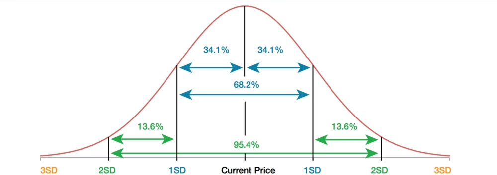
Now that you have the heavy lifting out of the way (working on the premise that you didn’t just type the STDEV into Excel instead of calculating it yourself…), you can make some inferences about the return profile, and future performance of the fund. In explanation of this newfound sentience, answers can be found on a normal distribution graph (you may recognize the “bell curve” diagram from school…). Now, the returns of investments do not always fit into the bell curve owing to their asymmetrical bias towards positive returns (called skew), but they will fall upon the curve often enough to render the exercise meaningful; particularly over longer time periods, using larger sample sizes.

Our fund has a mean monthly return of +1.025% and a standard deviation (volatility) of 3%. Based on this we can say that 68.2% of the time, over a 12 month period, a monthly return from the fund will be between-1.97% and +4.025%. Moving on, 95.4% of the time over a 12 month period, a monthly return from the fund will be between -4.975% and +7.025% and that 99.7% of the time the monthly returns will be between -7.975% and +10.025%. All in all, not a bad investment for somebody with a medium to long-term time horizon.The reliability of the inference that can be made is largely dependent upon the sample size, with more reliable conclusions being drawn from larger sample sizes with more data points (i.e investments which have longer track records and more performance history…). Even with sufficiently deep sample sizes there will be periods where performance is seemingly anomalous and at odds with our statistical predictions. Such goes the saying that “markets can remain irrational much longer than you can remain solvent”, however, if you are able to leave your capital committed you will likely realise performance which is in line with the long-term averages.

When flipping a coin there is a 50% probability of landing a head or a tails. This withstanding, you could flip the coin 5 times and get 5 heads. This does not mean that the coin is rigged or that the probabilities have changed from the original 50/50; it simply means that there have not been a sufficient number of occurrences for the probabilities to play out. If you were to flip the coin another 100 times you would move closer to a 50/50 distribution of heads and tails results as you move on. Probabilities are no guarantee of performance, nor are future results (which we base our probability assumptions on) any guarantee of future performance. Still, if you purchase an asset and it has a history of price appreciation over the long term, with a level of volatility that you are comfortable with, you should definitely hold the asset for as long as you can to benefit from the asymmetry of profit distributions.